Outline

• Introduction
• Markov Chains
• Metropolis-Hastings Algorithm
• Hamiltonian Monte Carlo
• Conclusion

Introduction

In this previous post, the Metropolis-Hastings and Hamiltonian Monte Carlo algorithms (HMC) were implemented using TensorFlow Probability without providing thorough details of the algorithms. This post explores the analytical and algorithmic details to provide data science practitioners with essential fundamentals that will illuminate the mechanics of these algorithms. To accomplish this, Markov chain theory is briefly reviewed followed by the mathematical details of Metropolis-Hastings and HMC and their implementation in python.

Markov Chains

Markov chains are defined as a sequence for random variables \(\small \small \left\{ \begin{array}{r} \theta^t, \theta^{t-1}, \ldots, \theta^0 \end{array} \right\}\) that follow the Markov property. This property states that for any time \(\small t\), the distribution of the random variable at time \(\small t\)depends only on the previous value. This can be formally expressed as

\(\small T_t\), the transition distribution, is a conditional distribution that defines the probability of a transition from state \(\small \theta^{t-1}\) to \(\small \theta^t\). When the state-space of the random variables is discrete, the transition distribution is a square matrix whose rows sum to one. If the transition matrix allows for any state to be reached from any other state and is not periodic then a unique stationary distribution exists. This can be trivially demonstrated using the Perron-Frobenius theorem on a subset of irregular, aperiodic matrices that assign positive probability to all states at any time \(\small t \; (T_{t-1, t}^t > 0)\). The Perron-Frobenius theorem states that such matrices will have an eigenvalue equal to one, it is the maximum eigenvalue, and its corresponding eigenvector will have strictly positive values. For state spaces that are not discrete, an additional condition must be satsified, namely, that the expected time to return to any state be finite. Demonstrating that the transition distribution or matrix meets these condtions is generally difficult; however, if it can be demonstrated that they are reversible, so long as there is positive probability to all states at any time, then there exists a stationary distribution. Reversibility is demonstrated if the detailed balance equations are satisfied, namely

To demonstrate that this condition preserves the distribution \(\small \pi\), one can sum over the states \(\small t-1\) and the following is obtained.

Thus a unique stationary distribution exists if:

1. The transition distribution is reversible and \(\small T_{t-1, t}^t > 0\)
2. The transition distribution allows for any state to be reached from any other state and is not periodic
3. If the state-space is continuous the expected time to return to any state be finite

Given the existence of unique stationary distributions for certain Markov chains, can one define a transition distribution such that the long-term behavior of the Markov chain is defined by a distribution one would like to draw samples from? The answer is clearly yes so long as the above conditions are met. This is the central idea behind MCMC methods; define a transition distribution such that a unique stationary distribution exists. The Metropolis algorithm was the first MCMC method that was implemented and it was discovered by physicists at Los Alamos in 1953. A generalized version of this algorithm came decades later and is known as the Metropolis-Hastings algorithm. The next section investigates the algorithm in detail and demonstrates that it constructs a transition distribution that meets the conditions for a unique stationary distribution to exist.

Metropolis-Hastings Algorithm

The Metropolis-Hastings algorithm specifies a transition distribution in two sperate steps: propose a value, \(\small \theta^*\) from a proposal distribution \(\small J_t(\theta^* \vert \theta^{t-1})\) and then accept the proposal according to another distribution \(\small r(\theta^* \vert \theta^{t-1})\). The algorithm proceeds as follows

1. Begin at an initial state \(\small \theta_0\) for which the target distribution, \(\small p(\theta \vert y)\), has positive probability
2. for \(\small t = 1, 2, ...\)
   • sample a proposal \(\small \theta^* \sim J_{t}(\theta^{*}\vert\theta^{t-1})\)
   • calculate the acceptance probability \(\small r(\theta^* \vert \theta^{t-1})=\text{min}\left(1, \frac{p(\theta^* \vert y)J_t(\theta^{t-1} \vert \theta^{*})}{p(\theta^{t-1} \vert y)J_t(\theta^* \vert \theta^{t-1})}\right)\)
   • set \(\small \theta^t = \theta^{*}\) with probability \(\small r(\theta^t \vert \theta^{t-1})\) otherwise set \(\small \theta^t = \theta^{t-1}\)

Random walks ensure that the expected return time is finite and they are non-periodic. If the proposal distribution is chosen such that it assigns positive probability to the entire continuous state space, then any state can be reached from any state. A commonly chosen distribution to ensure that these conditions are met is a multivariate normal distribution centered at the previous state, in other words, \(\small J_t(\theta^* \vert \theta^{t-1}) = \mathcal{N}(\theta^* \vert \theta^{t-1}, \Sigma)\). The only remaining condition to show is that the transition distribution, \(\small T_t(\theta^t \vert \theta^{t-1})\), is reversible. This is demonstrated by proving that two distinct points drawn from the target distribution have equal transition probabilities in either direction. Consider the points \(\small \theta_a\) and \(\small \theta_b \sim p(\theta \vert y)\) such that \(\small p(\theta_a \vert y)J_t(\theta_b \vert \theta_a) \leq p(\theta_b \vert y)J_t(\theta_a \vert \theta_b)\). This statement says that the probability of observing \(\small \theta_b\) is greater than that of a \(\small \theta_a\) (the sample \(\small \theta_b\) must be sampled from \(J_t(\theta^t \vert \theta^{t-1})\) and weighted against its probability distribution \(p(\theta^{t-1} \vert y)\)). If the transition distribution is reversible, then

The transition distribution is decomposed into its two components.

Because \(\small p(\theta_a \vert y)J_t(\theta_b \vert \theta_a) \leq p(\theta_b \vert y)J_t(\theta_a \vert \theta_b)\), the acceptance probability term on the left-hand side becomes one, thus

Thus, the transition distribution specified by the Metropolis-Hastings algorithm is reversible and a unique stationary distribution exists. If the algorithm is carried out sufficiently long, then the algorithm will converge to the unique stationary distribution and thus the accepted states will correspond to the target distribution \(\small p(\theta \vert y)\). To demonstrate how this algorithm can be implemented, a random walk transition distribution class and a function that advances the algorithm forward are created. The code block below displays the class and the function.

import numpy as np
import matplotlib.pyplot as plt
import autograd.numpy


class RandomWalkKernel(object):
    """Generate a proposal for the Metropolis-Hastings algorithm"""
    
    def __init__(
        self,
        target_log_prob_fn,
        init_state,
        cov,
        porposal_fn=None,
    ):
        self.cov=cov
        if porposal_fn is None:
            proposal_fn = sts.multivariate_normal
        self._proposal_fn = proposal_fn
        self._target_log_prob_fn = target_log_prob_fn
        
    def one_step(self, current_state):
        #at time t, the previous state is the current state from time t-1
        previous_state = current_state
        #propose a new state by adding gaussian noise to previous state 
        perturbation = self._proposal_fn(mean=np.zeros_like(previous_state), \
                                         cov=self.cov).rvs()
        proposed_state = previous_state + perturbation
        #calculate the proposed state log probability
        #log[p(theta*)]
        proposed_state_log_prob = self._target_log_prob_fn(proposed_state)
        #calculate the previous state log probability
        #log[p(theta^(t-1))]
        previous_state_log_prob = self._target_log_prob_fn(previous_state)
        #calculate the log acceptence correction factor(this value is 0 
        #when proposal function is symetric)
        #log[Jt(theta^(t-1)|theta*)/Jt(theta*|theta(t-1))]
        log_acceptence_correction = self._proposal_fn(mean=current_state, 
                                    cov=self.cov).logpdf(proposed_state) - \
        self._proposal_fn(mean=proposed_state, cov=self.cov).logpdf(current_state)
        #calculate log acceptance probability ratio 
        #log[p(theta*)Jt(theta^(t-1)|theta*)/p(theta^(t-1))Jt(theta*|theta^(t-1))]
        log_accept_ratio = proposed_state_log_prob - previous_state_log_prob + \
        log_acceptence_correction
        #calculate the minimum of 1 and log_accept_ratio
        r = min(1, log_accept_ratio)
        #draw a uniform random variable and transform to log space
        log_u = np.log(sts.uniform(0, 1).rvs())
        is_accepted = log_u < r
        #set current state at time t to proposal if accepted or previous state 
        #if rejected
        if is_accepted:
            current_state = proposed_state
        else:
            current_state = previous_state
            
        return current_state, is_accepted, log_accept_ratio, proposed_state

#Sampling function
def sample_markov_chain(n, init_state, kernel):
    states=[]
    results=[]
    current_state=init_state
    for i in range(n):
        current_state, is_accepted, log_accept_ratio, proposed_state = \
        kernel.one_step(current_state)
        states.append(current_state)
        results.append((is_accepted, log_accept_ratio, proposed_state))
        
    return states, results

All that is required to run the algorithm is to specify a target distribution, create an instance of the RandomWalkKernel class, and then call the function with the appropriate parameters. The code below shows how this is done with a multivariate isotropic normal distribution as the target distribution.

target_log_prob_fn = sts.multivariate_normal(mean=np.zeros(2), cov=1.).logpdf
init_state = np.array([-4., 4.])
kernel = RandomWalkKernel(target_log_prob_fn, init_state=init_state, cov=1.)
states, kernel_results = sample_markov_chain(100, init_state, kernel)

The image below shows three separate Markov chains with varying covariances, exploring the parameter space along with the corresponding traceplots. All three chains converge onto the region of high probability as expected.

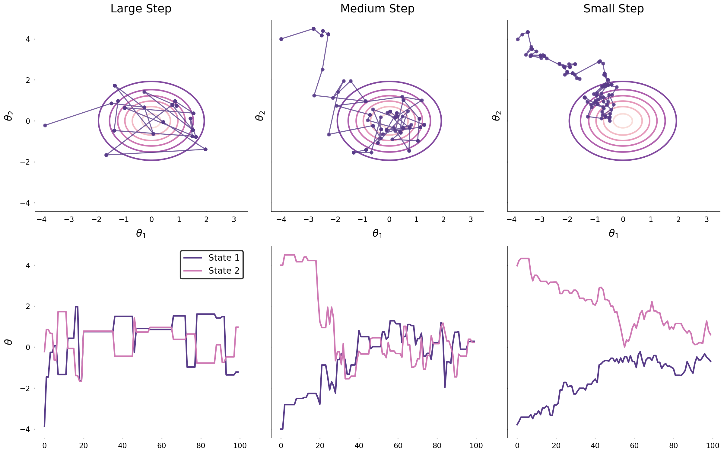
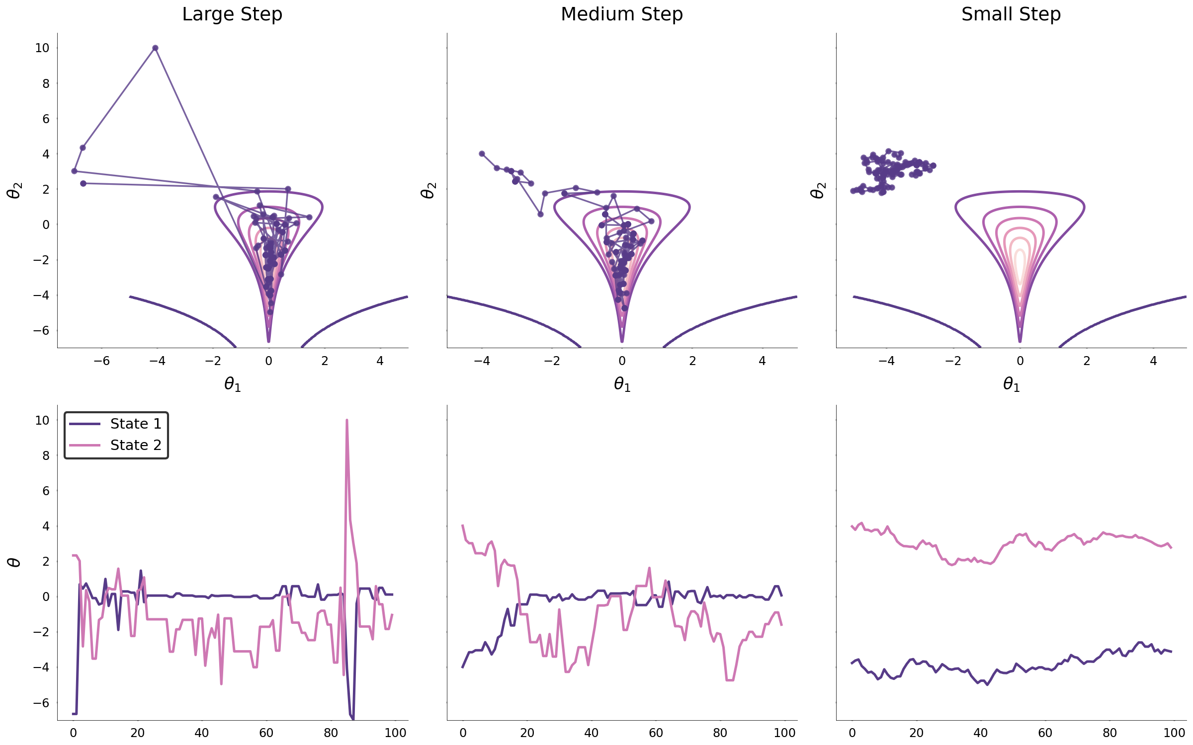
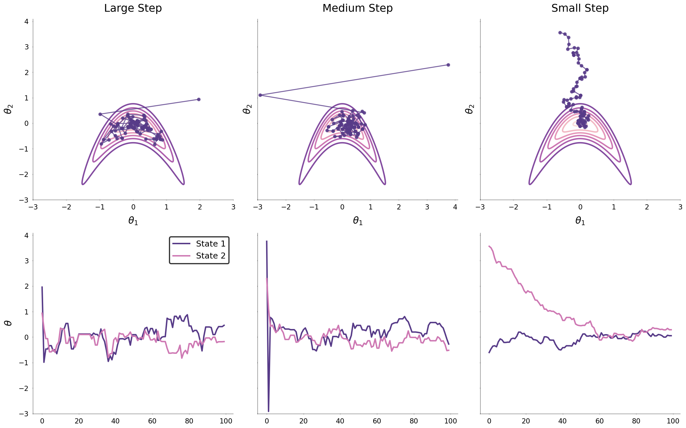
Unfortunately, in most problems of interest, the target distribution shape is far more complex than that of an isotropic multivariate normal. With increasing complexity, the covariance parameter becomes far more important for the efficient exploration of parameters space. The two images below display the same process for a funnel and a parabolic distribution.

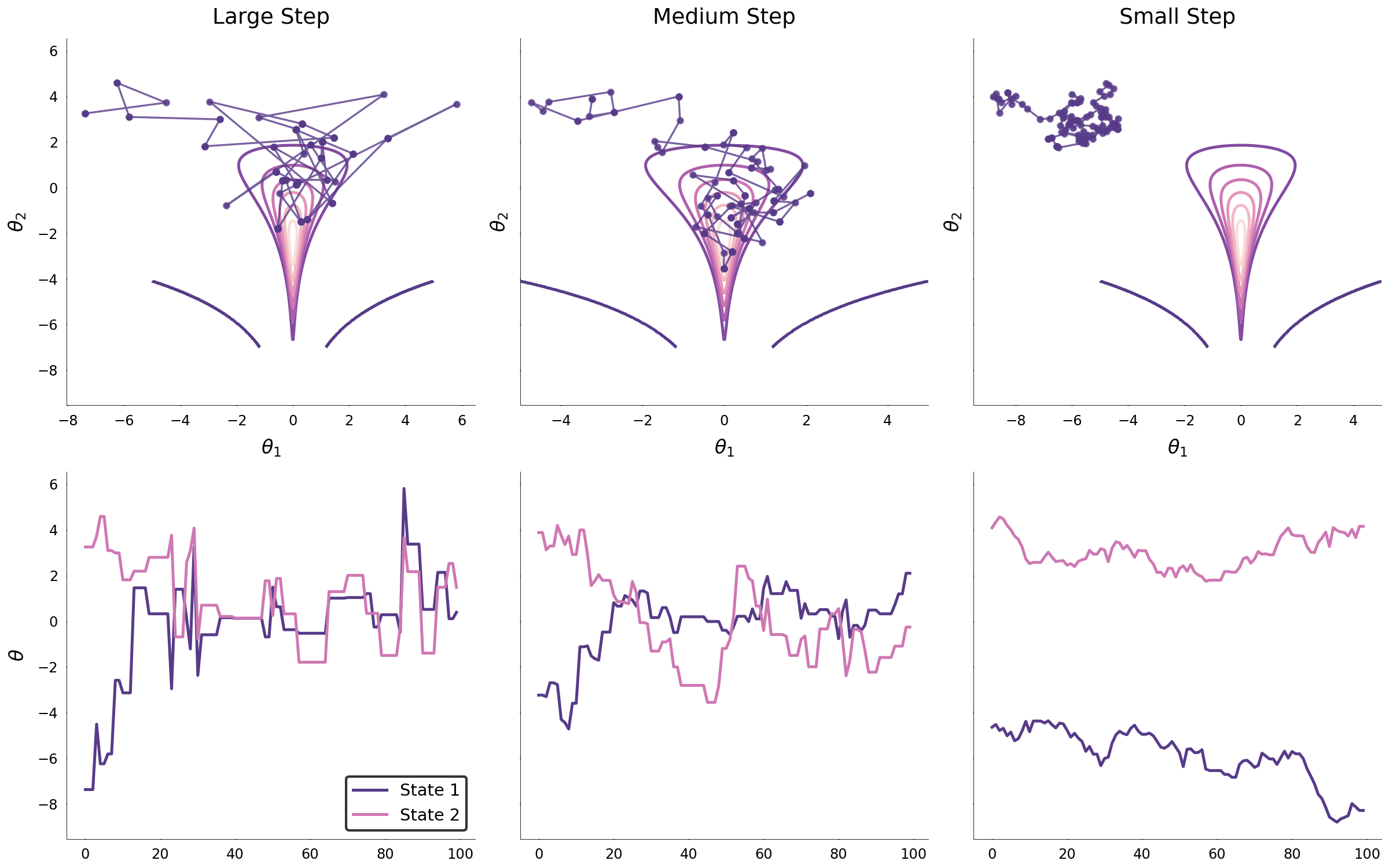
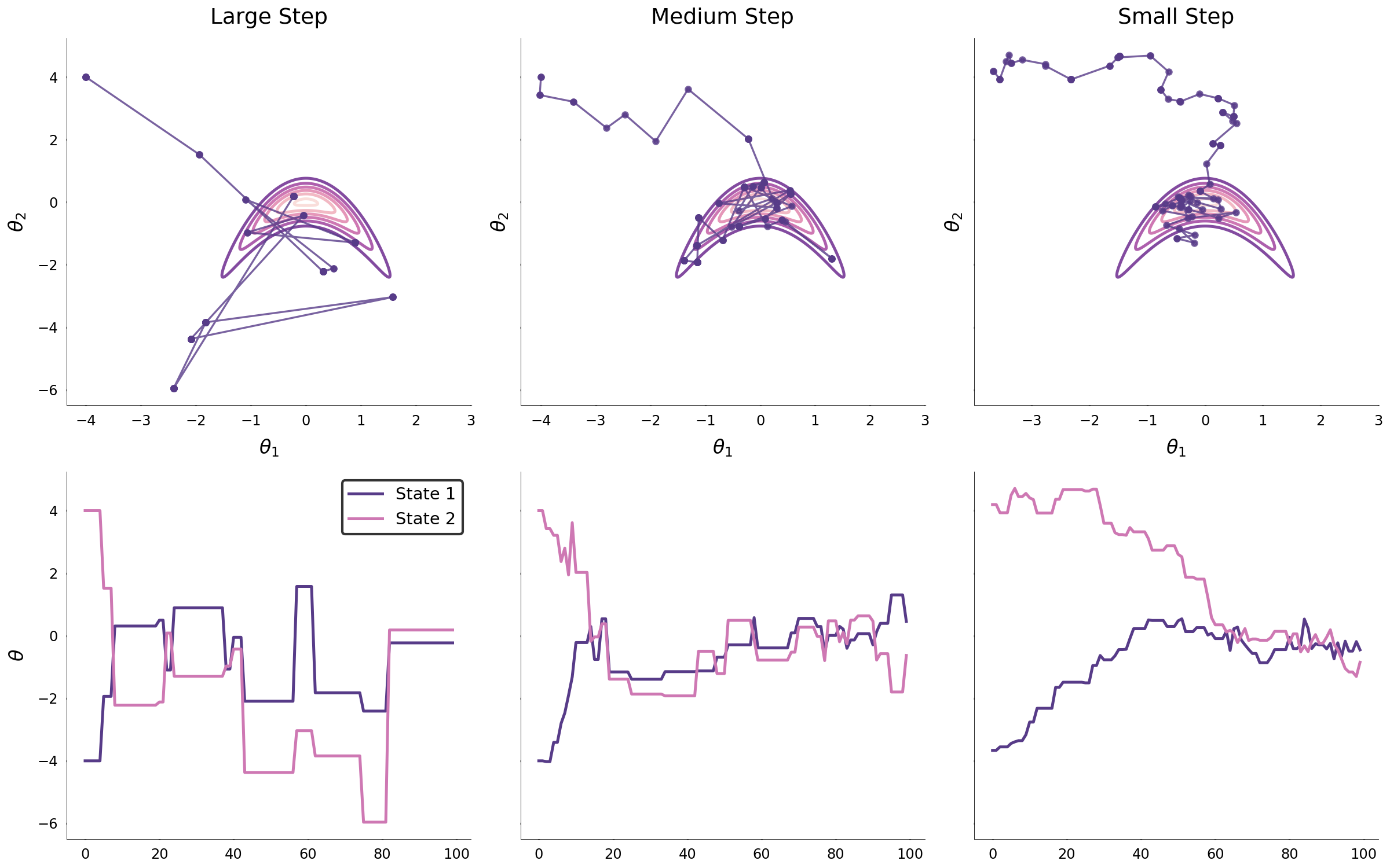
When the step size is large, it may be that the Markov chain converges to the target distribution rapidly; however, the large step size prohibits from efficiently exploring the high density region. Similarly, small step sizes may lead to a slow convergence and to inefficient exploration of regions of high probability density. One might conclude that so long as the step size is properly tuned, that the target distribution will be explored efficiently. While this may hold in low-dimensional spaces, when the dimensionality of target distribution is large, the random walk behavior of the Markov chain will likely always propose parameters outside of the region of high probability. The reason why this occurs in high dimensional spaces is because the volume outside the target distribution grows exponentially with the dimensionality. Thus, it is likely that the random walk Markov chain explores the large volume outside the target distribution which limits the application of the Metropolis-Hastings algorithm.

Auxiliary variables can be introduced to drastically improve efficient exploration of an augmented parameter space \(\small (\theta, \phi)\), where \(\small \phi\) is the auxiliary variable. If \(\small p(\theta, \phi)\) is easier to sample than \(\small p(\theta)\) and \(\small \int_{\phi}p(\theta, \phi)d\phi = p(\theta)\), then the samples \(\small \theta\) can be easily recovered. One such method that uses auxiliary variables is HMC. HMC is more difficult to understand because it borrows ideas from physics which many data science practitioners may be unfamiliar with and thus may find it to be unappealing. However, the applicability of HMC on complex and high-dimensional problems makes it an extremely valuable tool and thus warrants a thorough understanding. A key to understanding how this algorithm works and why it is efficient in high-dimensional spaces is to explore HMC from an analytical and intuitive perspective. The following section begins by presenting HMC from an intuitive perspective followed by the analytical framework that validates the HMC algorithm as a MCMC method and its implementation.

Hamiltonian Monte Carlo

HMC expands the parameter space \(\small \theta\) to \(\small (\theta, \phi)\), generates proposals by advancing the tuple \(\small (\theta, \phi)\) for some time using Hamiltonian dynamics, and then accepting or rejecting the proposal as in the Metropolis-Hastings algorithm. The key to efficient exploration lies within the use of Hamiltonian dynamics to generate proposals. Hamiltonian dynamics describes the evolution of the state of classical systems which consists of its position and momentum. If the Markov chain exploring parameter space is thought of as a frictionless particle moving about a surface specified by the target distribution, ideally, the Markov chain should explore regions that contribiute significantly for an accurate approximation of the target distribution. So how can one inform the Markov chain to account for this? A straightforward solution is to add information about the gradient of the target distribution because it will define a vector field over parameter space that will keep the Markov chain away from the non-informative volume outside the target distribution associated with high dimensional spaces. For simplicity, consider that the Markov chain is exploring a parameter space that is shaped like a bowl. The associated vector field is flat in regions away from the mode and increasingly steep towards the mode. If the Markov chain is initially in a region of low probability, then as time evolves the Markov chain will traverse directly towards the mode, and ultimately remain at equilibrium at the mode. This demonstrates that adding a vector field defined by the gradient of the target distribution is not sufficient.

The physical analog of the gradient of an MVN can be thought of as a planet’s gravitational field pulling objects towards its center. Despite the gravitational field of a planet, many planets have objects that remain in orbit and do not spiral towards the center of the planet or into the vastness of space. This is due to the associated momentum of the object that allows it to overcome the gravitational force in such a way that it remains in orbit about its planet. Such systems are known as conservative systems. This motivates the idea that the Markov chain must be endowed with sufficient momentum as to overcome the gradient yet not be cast off into the vast volume outside the target distribution. The only method that endows the probabilistic system with the precise momentum is HMC. This is because Hamiltonian dynamics exhibit special mathematical properties that keep the target distribution invariant and thus the Markov chain specified by HMC ensures that a unique stationary distribution exists. These properties are reversibility, volume preservation, and conservation of the Hamiltonian.

Hamiltonian dynamics specify a mapping that advances the tuple \(\small (\theta^{t-1}, \phi^{t-1})\) forward in time to \(\small (\theta^t, \phi^t)\) and are defined as follows

For HMC, the Hamiltonian, \(\small H(\theta, \phi)\), is specified as

These are the sum of potential and kinetic energies of the system. Note that the kinetic energy term is quadratic with respect to \(\small \phi\) thus \(\small K(\phi) = K(-\phi)\). To demonstrate that this mapping leaves the target distribution invariant, negating the derivatives with respect to time must equal their positive counterparts. With respect to the Hamiltonian, to negate time, one must negate the momentum. Thus,

and

This proves that Hamiltonian dynamics are reversible and thus preserve the target distribution. Just like how an object can orbit a planet by balancing the potential and kinetic energies, the probabilistic system must also mimic a conservative system to ensure that the Markov chain does not converge towards equilibrium or diverge away from the target density. Conservative systems require that volumes be exactly preserved and thus Hamiltonian dynamics must preserve volume to endow the probabilistic system with the correct momentum. It can be shown that vector fields with zero divergence preserve volume. The divergence of the vector field is taken as follows.

Hamiltonian dynamics are both reversible and preserve volume thus will preserve the target distribution and will mimic a conservative system. Another property that is important is that the Hamiltonian is kept invariant. This can be shown by taking the time derivative of the Hamiltonian and showing that it is zero.

Having demonstrated that Hamiltonian dynamics preserve the target distribution and that they mimic a conservative system and thus can be used to sample from \(\small p(\theta, \phi)\), the next step is to incorporate the Hamiltonian operator with the joint distribution. This is done by using the concept of a canonical distribution from statistical mechanics. The canonical distribution will relate the potential energy of the probabilistic system to the target distribution. The canonical distribution is

This distribution gives the probability of a state \(\small x\) of a physical system according to an energy function \(\small E(x)\). The terms \(\small Z\) and \(\small T\) are the normalizing constant and temperature of the system, respectively. Moving forward, the normalizing constant will be ignored for convenience and the temperate of the system will equal one. The state of the probabilistic system consists of the position-momentum tuple \((\theta, \phi)\) whose energy is specified by the Hamiltonian operator \(\small H(\theta, \phi)\). Substituting these terms into the canonical distribution yields

If the joint probability distribution is factorized, then

This demonstrates how the target distribution is related to a potential energy function that is independent of the auxiliary momentum variable. Furthermore, the factorization of the joint distribution implies that the momentum variable can be marginalized and thereby recovering the target distribution. In practice, the distribution \(\small p(\phi \vert \theta) = \mathcal{N}(0, M^{-1})\), where \(\small M^{-1}\) is known as the mass matrix and is typically an identity matrix scaled by some constant. Expanding the parameter space is done by sampling from this distribution and then Hamiltonian dynamics are simulated to generate a proposal. The acceptance probability is then evaluated according to the acceptance probability defined by the Metropolis-Hastings algorithm shown below.

This can be equivalently expressed as the log acceptance probability

HMC can then be implemented as follows:

1. Sample the auxiliary momentum \(\small \phi \sim \mathcal{N}(0, M^{-1})\)
2. Advance the position/momentum tuple \(\small (\theta^{t-1}, \phi{t-1})\) forward in time according to \(\small \frac{\partial H(\theta, \phi)}{\partial \phi}, -\frac{\partial H(\theta, \phi)}{\partial \theta}\) to propose a new state \(\small (\theta^*, \phi^*)\)
3. Accept the proposal with probability \(\small \log r(\theta^*, \phi^*)\) otherwise reject.

When simulating Hamiltonian dynamics, Hamilton’s equations must be approximated by discretizing time. Typically, this is done via the leapfrog method and works as follows:

First, a half step is advanced forward for the momentum vector, followed by a full step for the position vector with the updated momentum, and finally another half step for the momentum vector using the updated position vector. The leapfrog method also preserves volume exactly and is reversible. Reversibility is applied by negating the momentum, applying a specified number of steps and then negating the momentum at the end. With this, the HMC can be implemented as follows.

class HamiltonianMonteCarlo(object):
    """Runs one step of Hamiltonian Monte Carlo"""
    
    def __init__(
        self,
        target_log_prob_fn,
        step_size,
        num_leapfrog_steps,
    ):
        
        self._target_log_prob_fn = target_log_prob_fn
        self.step_size = step_size
        self.num_leapfrog_steps = num_leapfrog_steps
        
    def one_step(self, current_state):
        
        #helper function that returns auxiliary momentum variables 
        def momentum_sampler(shape):
            return sts.multivariate_normal(mean=np.zeros(shape)).rvs()
        
        #leapfrog integrator
        def leapfrog_integrator(current_momentum, current_state):
            current_state, current_momentum = np.copy(current_state), \
            np.copy(current_momentum)
            #derivative of potential function
            dHdq = elementwise_grad(self._target_log_prob_fn)
            #advance momentum half step
            current_momentum +=  self.step_size * dHdq(current_state) / 2
            #loop for specified leapfrog steps leaving one step for final
            #momentum half step
            for i in range(self.num_leapfrog_steps - 1):
                #advance position full step
                current_state += self.step_size * current_momentum
                #advance momentum full step 
                current_momentum += self.step_size * dHdq(current_state)
            current_state += self.step_size * current_momentum
            current_momentum += self.step_size * dHdq(current_state) / 2
            #momentum flip at the end to ensure reversibility
            return current_state, -current_momentum
        
        shape = current_state.shape
        #at time t, the previous state is the current state from time t-1
        previous_state = current_state
        #draw auxiliary momentum variable
        previous_momentum = momentum_sampler(shape)
        #generate proposal by simulating Hamiltonian dynamics
        proposed_state, current_momentum = leapfrog_integrator(previous_momentum, 
                                                               current_state)
        #sum of kinetic energies
        log_acceptence_correction = np.sum(current_momentum ** 2 - \
                                           previous_momentum ** 2) / 2
        #sum of potential energies
        proposed_state_log_prob = self._target_log_prob_fn(proposed_state) - \
        self._target_log_prob_fn(previous_state)
        #log probability of acceptance 
        log_accept_ratio = proposed_state_log_prob + log_acceptence_correction
        #log acceptance ratio
        r = min(1, log_accept_ratio)
        #Metropolis step
        log_u = np.log(sts.uniform(0, 1).rvs())
        is_accepted = log_u < r
        if is_accepted:
            current_state = proposed_state
        else:
            current_state = previous_state
        return current_state, current_momentum, previous_momentum, is_accepted, log_accept_ratio

#sampling function
def sample_hmc_markov_chain(n, init_state, kernel):
    states=[]
    results=[]
    current_state=init_state
    for i in range(n):
        current_state, current_momentum, previous_momentum, is_accepted, log_accept_ratio = \
        kernel.one_step(current_state)
        states.append(current_state)
        results.append((current_momentum, previous_momentum, is_accepted, log_accept_ratio))
        
    return states, results

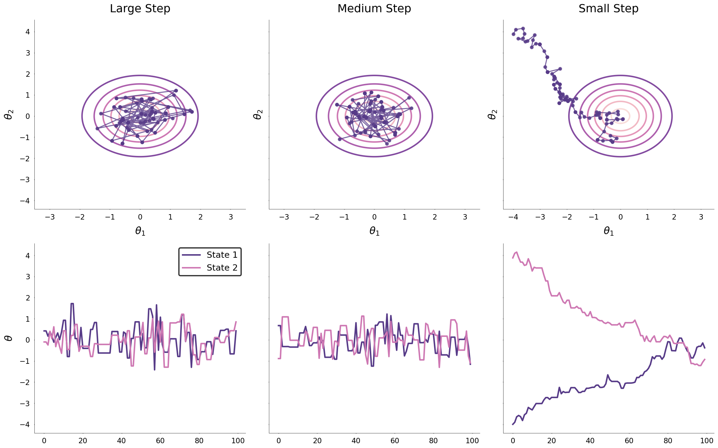
The algorithm is used to build three Markov chains to explore the same distributions that were explored using the Metropolis-Hastings algorithm. Analogous to the covariance parameter in the Metropolis-Hastings algorithm, the number of leapfrog steps and the step size will dictate how efficiently the Markov chain converges to the target distribution and explores it. Its difficult to demonstrate the efficiency of HMC with simple two-dimensional examples; however, by introducing the auxiliary momentum variables, proposals can be generated by simulating Hamiltonian dynamics which efficiently explore the canonical distribution through a vector field that corresponds to the target distribution.

Conclusion

By leveraging the fact that irreducible, aperiodic, non-null recurrent Markov chains have a unique stationary distribution, Markov chain Monte Carlo methods specify valid transition distributions that will allow for any target distribution to be sampled. The Metropolis-Hastings algorithm accomplishes this by specifying a reversible transition distribution that explores parameter space via a random walk. Because of the large volume outside the target distribution in high dimensions, the Metroplis-Hastings algrotihm is inneficient. HMC is an auxiliary MCMC method that effciently explores the target distribution by borrowing concepts from physics.